This post describes the process of developing a end-to-end Machine Learning model to steer an RC Car around using a color camera as an input. This is inspired by the Udacity Self Driving Car “behavior cloning” module as well as the DIY Robocars races.

The purpose of this project is to create a pipeline for collecting and processing data as well as training and deploying a ML model. Once that basic infrastructure is in place, we can build upon that foundation to tackle more challenging projects.

For this project, the goal is to develop a ML model that reliably navigates the RC car around a racetrack. The ML model will perform a regression to estimate a steering angle for each camera image. We will test everything in simulation using ROS Gazebo and then use the same system to drive autonomously around an indoor track in the real world.

Data Collection in Simulation

We will first use a simulated environment to validate the data pipeline, model training, and model deployment process. We will use ROS Gazebo as the simulation environment and visualize the camera output in RViz.

Simulation Environment Setup

To generate simulated images, we will use a simulated RGB color camera. The camera will be mounted on a simulated RC car provided by the MIT RACECAR project.

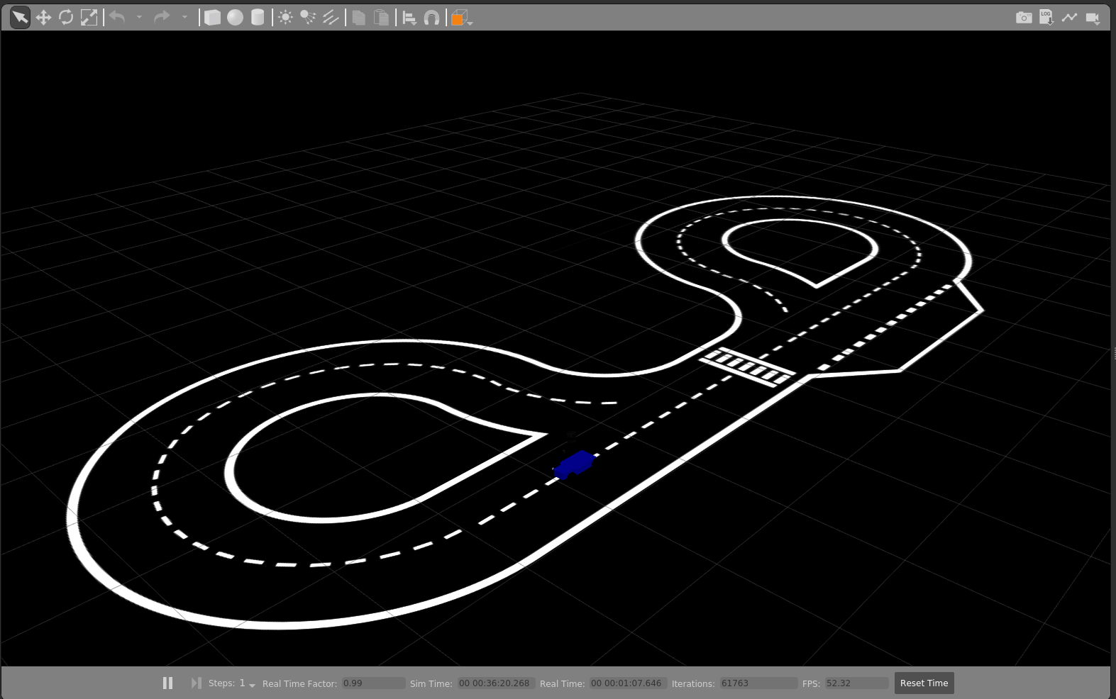
Lastly, we will use the Conde world file developed by Valter Costa for his paper, “Autonomous Driving Simulator for Educational Purposes” as the simulated environment to operate the system and serve as a test track for training. The package for the Conde model is available here, and should be saved in the default Gazebo world directory ~/.gazebo/model. You can verify that the model loads correctly by loading it in Gazebo as shown below.

A sample image of the RGB camera mounted on the racecar platform in the Conde Gazebo environment is below:

Simulated Data Collection

In order to train our ML model, we will need a labeled data set. The project is known as behavior cloning because we want to manually drive the vehicle around the track and train an ML model to copy that behavior. Therefore, to create a training data set, we will manually drive the simulated vehicle around the track, trying to stay as close as possible to the centerline of the track. We will record each image as well as the steering commands given to the vehicle.

To run the simulation environment, we will use the rc_dbw_walker.launch launch file and pass the world_name argument. This will generate the RC car with the simulated camera in the Conde world. This will also spawn several nodes which allow us to control the vehicle’s steering and throttle with a remote controller.

$ roslaunch rover_gazebo rc_dbw_walker.launch world_name:=conde_world

Once the simulation is loaded, we will begin recording data. The record_training.sh script is used to record the following topics:

– /racecar/ackermann_cmd_mux/output
– /openmv_cam/image/raw

The script also splits bags into 1 GB files and applies lz4 compression. The file will be prefixed with ‘ml_training’ followed by the timestamp of the bag.

Once the system is recording, drive the vehicle around the track for a couple of laps, keeping the vehicle as close as possible to the center lane of the track.

ROS bag File Processing

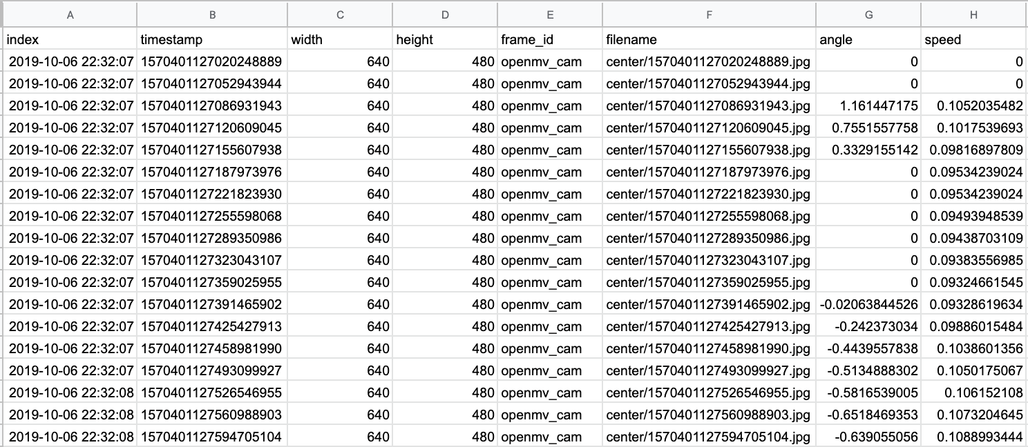
Once we’ve collected the training data, we need to organize and process it. We want to extract the camera data and steering data from the ROS bag and save it in a format that is easier to manipulate. We will save the camera images as JPG files with unique filenames based on the timestamp they were recorded. We also extract the steering commands which are stored in a CSV file. Each row in the CSV file lists the image filename as well as the steering and throttle values associated with that image.

To execute the transformation, we will use the rosbag_to_csv.py. This is a slightly modified version of Ross Wightmans bagdump.py script.

$ python rosbag_to_csv.py -o output/walker/ -i data/walker/

This CSV file (interpolated.csv) and the associated JPG images form the basis of our training data set. An example of the CSV output is shown below.

Train and Test the ML Model

To train the model, we will be using the TensorFlow, Keras, and sklearn libraries. The training process is executed by the model_train.py script.

We use the CSV file generated previously as the basis of our dataset. This CSV file contains the image filenames which we will use for features and the recorded steering angle which will be the label.

Create Training and Validation Data Sets

Our first step is to shuffle and split the dataset into a training set and a validation set. We use sklearn functions to create two arrays, train_samples and validation_samples.

sklearn.utils.shuffle(samples)

train_samples, validation_samples = train_test_split(samples, test_size=0.2)

The number of samples in each set is output. For my dataset, I had the following split:

('Number of training samples: ', 364)
('Number of validation samples: ', 121)

Define a data generator

When working with large datasets, it’s helpful to use Keras data generators to handle loading the data. These are specifically helpful when manipulating datasets containing images. For this example, we will define our own basic data generator. In the future, we can use the Keras implementations such as the ImageDataGenerator class.

Our data generator will take in a dataset of sample data as well as the batch size hyperparameter value and a flag to determine if the data should be augmented.

def generator(samples, batch_size=32, aug)

The data generator begins by loading a specific set of data from the samples based on the batch size

batch_samples = samples[offset:offset + batch_size]

For each sample, it loads an image and resizes it.

center_image = cv2.imread(name)
center_image = cv2.resize( center_image, (320, 180))

It then loads the steering angle associated with that image.

angle = float(batch_sample[6])

The image and the angle are then stored in unique arrays:

images.append(center_image)
angles.append(angle)

If the aug flag is enabled, we perform basic image augmentation. For this example, we flip the image as well as the angle and store those values into the arrays.

flip_image = np.fliplr(center_image)
flip_angle = -1 * angle
images.append(flip_image)
angles.append(flip_angle)

Lastly, we shuffle and return the arrays.

yield sklearn.utils.shuffle(X_train, y_train)

We define the batch size hyperparameter and then create our training and validation data generators.

batch_size_value = 32

train_generator = generator(train_samples, batch_size=batch_size_value, 1)
validation_generator = generator(validation_samples, batch_size=batch_size_value, 0)

Model Architecture and Training

For this application, we will use the model developed by Nvidia and described in their blog post, “End-to-End Deep Learning for Self-Driving Cars.” The model is defined in their paper, “End to End Learning for Self-Driving Cars.” They develop a convolutional neural network (CNN) to map raw pixels from a single front-facing camera directly to steering commands.

The network consists of 9 layers, including a normalization layer, 5 convolutional layers and 3 fully connected layers. A visualization of the model from the paper is shown below:

This model is compiled using the following keras functions.

First, we define the model as a sequential model.

model = Sequential()

Next, we trim the input image so we are only focused on the bottom portion of the image which contains the road and lane markings.

model.add(Cropping2D(cropping=((75, 0), (0, 0)), input_shape=(180, 320, 3)))

We also perform some basic preprocessing of the incoming data. We normalize the image values centered around zero with small standard deviation.

model.add(Lambda(lambda x: (x / 255.0) - 0.5))

The remaining lines define the specific model layers.

model.add(Cropping2D(cropping=((0,0), (0,0)), input_shape=(180,320,3)))
model.add(Convolution2D(24, (5, 5), activation="relu", name="conv_1", strides=(2, 2)))
model.add(Convolution2D(36, (5, 5), activation="relu", name="conv_2", strides=(2, 2)))
model.add(Convolution2D(48, (5, 5), activation="relu", name="conv_3", strides=(2, 2)))
model.add(SpatialDropout2D(.5, dim_ordering='default'))
model.add(Convolution2D(64, (3, 3), activation="relu", name="conv_4", strides=(1, 1)))
model.add(Convolution2D(64, (3, 3), activation="relu", name="conv_5", strides=(1, 1)))
model.add(Flatten())
model.add(Dense(1164))
model.add(Dropout(.5))
model.add(Dense(100, activation='relu'))
model.add(Dropout(.5))
model.add(Dense(50, activation='relu'))
model.add(Dropout(.5))
model.add(Dense(10, activation='relu'))
model.add(Dropout(.5))
model.add(Dense(1))

This results in a model with 15,004,791 trainable parameters.

Next, we set up a callback function that will be executed during the model training process. Specifically, we set up checkpoints using the following function.

checkpoint = ModelCheckpoint( filepath, monitor='val_loss', verbose=1, save_best_only=True, mode='auto', period=1)

This gets added to a callback list.

callbacks_list = [checkpoint]

As the model is training, this function stores the weights of the model with the highest performance at the time. If the training process gets interrupted, we can load these model weights and continue training the model without having to start from scratch.

Once the callbacks are properly initialized, we set the hyperparameters.

First, we define the step sizes for the training and validation data.

steps_per_epoch=(len(train_samples) / batch_size_value)
validation_steps=(len(validation_samples) / batch_size_value)

This defines the total number of steps (batches of samples) to yield from the data generator before declaring one epoch finished and starting the next epoch.

Next, we set the number of epochs.

n_epoch = 30

Finally, we use the fit_generator function to start the model training process.

history_object = model.fit_generator( train_generator, steps_per_epoch=(len(train_samples) / batch_size_value), validation_data=validation_generator, validation_steps=(len(validation_samples) / batch_size_value), callbacks=callbacks_list, epochs=n_epoch)

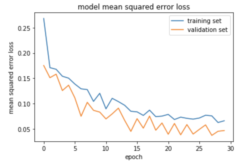
Model Evaluation

Once the model is finished training, we want to evaluate its performance. We can plot the loss values for the training and validation data sets across the epochs.

Model Deployment and Verification

Once the model is trained, we want to verify the model performance in simulation. We will place the simulated RC car back in the Conde environment but we will rely on the output of the ML model to determine the appropriate steering command.

ML Model Inference ROS node

Next, we need to develop a ROS node that subscribes to the image topics published by the camera and published the control commands that are output from the ML model. The drive_model.py file is used to do this.

The model_control_node is created which subscribes to the /openmv_cam/image/raw topic for camera images and publishes control commands on the /platform_control/cmd_vel topic.

The model we trained is loaded using the Keras load_model() function.

model = load_model('/behavior_cloning/model.h5')

When an image is received, we use the cv_bridge package to transform the image data from the ROS message type to a OpenCV image.

bridge.imgmsg_to_cv2(data, "bgr8")

For each image received, it is first resized to a 180×320 image. This is the image size that we trained the model on and this is the format that the model expects for inputs.

self.resized_image = cv2.resize(self.latestImage, (320,180))

Next, the image is converted into a numpy array.

image_array = np.asarray(self.resized_image)

For this project, we are only concerned with estimating the steering angle of the RC car. Therefore, we hard code the throttle at a constant value.

self.cmdvel.linear.x = 0.13

Next, we provide the input image to the ML model and it returns a predicted steering angle.

self.angle = float(model.predict(image_array[None, :, :, :], batch_size=1))

We limit the predicted output to the maximum steering inputs allowed by the vehicle.
self.angle = -1.57 if self.angle < -1.57 else 1.57 if self.angle > 1.57 else self.angle

Finally, we set the steering angle command to the estimated value

self.cmdvel.angular.z = self.angle

and publish the desired throttle and steering angle commands

self.cmdVel_publish(self.cmdvel)

The system completes this prediction loop continuously to provide updated steering angle commands to the vehicle.

ML Model Simulated Deployment

In order to run the drive_model.py ROS node, we need to add the following to our rc_dbw_walker.launch launch file.

<node name="behavior_cloning_node" pkg="behavior_cloning" type="drive_model.py" output="screen" respawn="true"/>

Once we execute that launch file, the drive_model.py ROS node will begin processing images from the simulated camera and outputting desired steering angles on the /platform_control/cmd_vel topic.

The image below shows the vehicle navigating the Conde world using the output of the trained ML model. While the vehicle isn’t perfectly centered in the lane, this does verify that the model is predicting accurate steering commands and the overall system performance is validated.

Real-world Performance

Once the data collection, processing, training, and deployment pipeline is validated in simulation, we can test the process in a real-world environment. For this example, we will mount a Genius WideCam F100 webcam to the RC platform. The system also has an Ouster OS1-64 mounted which is not used for this application. The vehicle can be operated remotely with an Xbox controller. All processing is done on a fitlet2 with an Arduino Uno providing commands to the motors for steering and throttle. This set-up closely mimics the simulated system used earlier.

Training Data Collection

When manually operating the RC car, the rc_dbw_cam.launch launch file is used to start the system.

$ roslaunch rover_teleop rc_dbw_cam.launch os1:=false ekf:=false

As before, we use the record_training.sh script to record the training data.

$ source record_training.sh

For this data collection period, we want to try to get at least 10,000 labeled images for training. I manually drove the vehicle around the track 5 times, reversed directions, and drive for 5 more laps. An example of the collected video is shown below.

The collection of ROSbags was then processed to extract individual images and steering angles using the rosbag_to_csv.py script. This resulted in a local directory of images and an interpolated.csv file correlating image file names with the associated steering angle.

Model Training and Deployment

Once the training data was processed, the model_train.py script was used to split the data into training and validation data sets. It then compiled and trained the Nvidia end to end CNN and generated a model file.

 

Model Deployment

Once the model was trained, the drive_model.py file was updated with the path to the new model file. This file creates the ROS node which loads the model and uses the incoming images from the webcam to infer the desired steering angle.

To launch the complete system, the rc_mlmodel_cam.launch is used. This launch file loads the drive_model.py ROS node in addition to loading the common RC vehicle input and control nodes defined in rc_dbw_cam.launch.

When the system is running, the vehicle can be controlled by two different inputs. The control commands from the Xbox controller are still subscribed to on the /joy_teleop/cmd_vel topic. Additionally, the ML model is publishing control commands on the /platform_control/cmd_vel topic.

We use the yocs_cmd_vel_mux node which serves as a multiplexer for command velocity inputs. It arbitrates incoming cmd_vel messages from several topics, allowing one topic at a time to command the robot, based on priorities. All topics, together with their priority and timeout are configured through a YAML file, that can be reload at runtime. This is defined in the rover_cmd_vel_mux.yaml configuration file.

Once the system is properly configured, the RC vehicle is placed on the track and the system is executed using the rc_mlmodel_cam.launch launch file.

$ roslaunch behavior_cloning rc_mlmodel_cam.launch

The video below depicts a completely autonomous lap using the model defined in this process. The image recorded by the webcam can be seen as well as an overlay of the saliency image depicting the areas in the image that most contribute towards the steering command output.