Previously, the process for training and deploying an ML model to autonomously operate an RC car was described in the post, “RC Car End-to-end ML Model Development.” The purpose of the project was to develop an ML model that predicted steering angles given a color camera image input to enable the RC car to follow a lane around a track autonomously. A video of the real-world implementation of this model is depicted below.

This post describes the process of using Google Colab for the model training process instead of the embedded device on the RC car. Google Colab is a free research tool for machine learning education and research. It’s a Jupyter notebook environment that can be accessed via a web browser. Code is executed in a virtual machine and the notebook files are stored in your Google Drive account. For this example, everything will be done in Python.

Depending on the size of the dataset or the complexity of the model, it can be difficult to train an ML model on an embedded device. Google Colab offers free use of GPUs and now provides TPUs as well. The virtual machines also have 12GB of RAM and 320GB of disk space. This makes them a great tool for training ML models with large data sets.

Environment Setup

This section describes the steps required to collect a training dataset and prepare the Google Colab notebook environment.

Data Collection

This tutorial assumes that training data is already collected and available. The post, “RC Car End-to-end ML Model Development” describes the process of manually operating an RC car running ROS to collect training data. An example of that data is shown below.

The post also described how to take the camera images and associated steering commands collected in ROS and transform them into a dataset ready to be used for ML model training. The dataset is available here.

Google Colab Setup

We will use the RC Car End-to-End Image Regression with CNNs (RGB camera).ipynb notebook to process the dataset, train the ML model, and evaluate the ML model’s performance. First, we want to make sure the runtime environment is properly setup. From the Runtime menu, select the option to Change runtime type to get to the Notebook settings modal.

The notebook is compatible with Python 2 or Python 3 but make sure the GPU is selected in the Hardware Accelerator dropdown.

Once the notebook is properly setup, we can begin executing the notebook. The first cell imports all the libraries needed for the execution of the notebook. The notebook is not compatible with TF2.0 at this time. The command %tensorflow_version 1.x ensures that TF1.0 is used instead of TF2.0. The cell outputs the Tensorflow and Keras versions loaded.

Tensorflow Version: 1.15.0
Tensorflow Keras Version: 2.2.4-tf
Eager mode: False

Finally, we confirm that the GPU we selected is available. If the GPU is available, the name is also printed. Currently, a Nvidia Tesla P100 is available.

Load the Dataset

Once the notebook is properly configured and the environment setup, we can start loading the dataset to be used for training. The dataset is stored as a .tar file hosted on AWS. The dataset is downloaded and extracted into the Colab environment.

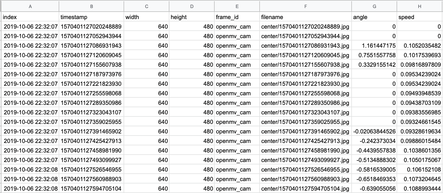
In the Files tab, we can view the structure of the dataset directory. The center directory contains all the image files. The steering.csv file contains data about the steering commands and the camera.csv file contains data about each of the images. The interpolated.csv file combines the image and steering information into a single file. Since the camera and the steering commands occur at different frequencies, the interpolated.csv file contains an estimate of a steering command for each image. An example of the file is shown below.

Next, we parse the interpolated.csv file and load the information into a Pandas dataframe. This format makes it easier to manipulate since Pandas has a lot of helper functions for handling data. A summary of the dataframe is provided as the cell output.

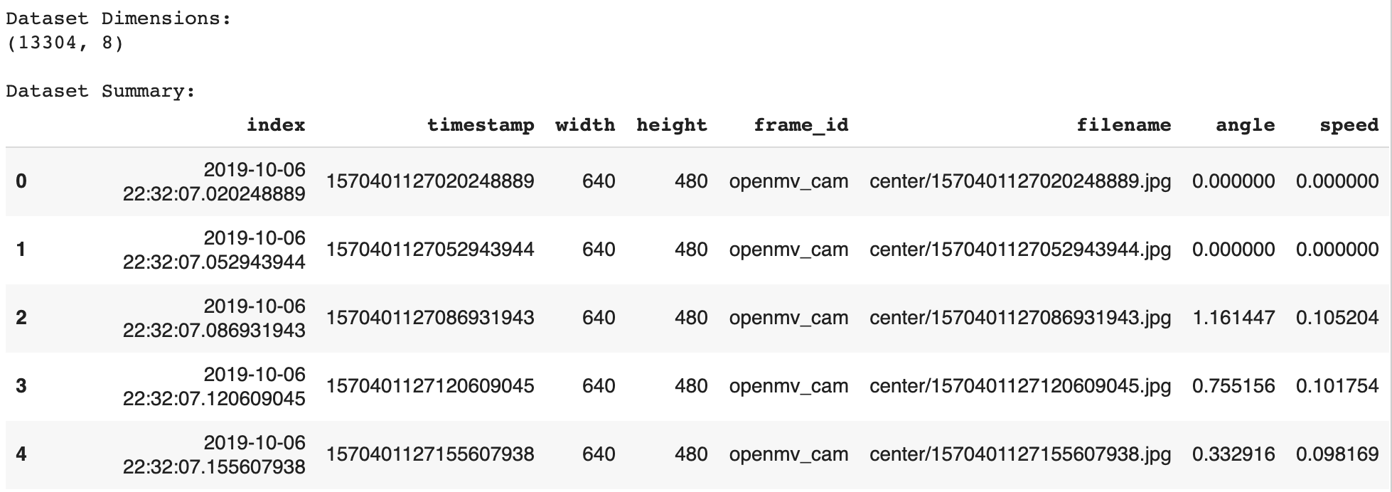
This dataset has over 13,000 samples and contains the same data as the interpolated.csv file.

Pre-process the Dataset

Once the data is loaded into a dataframe, we can run some basic quality to checks to clean the data. After removing some extraneous columns, we look for and remove any entries will NULL values.

We also remove any entries where the speed value is 0. We only want the model to be trained on data where the RC car was moving. This removes a few entries, but nothing significant.

We can also print some basic statistics about the dataset.

We know the min and max values allowed on the vehicle are +/- 1.54 so the min and max values of the dataset look acceptable. The course also primarily consisted of right-hand turns, so a mean and median value above 0 also makes sense.

We can visualize the distribution of the steering commands using a histogram. The widget allows the user to select the number of bins to use of the histogram. Using the default of 25 bins produces the histogram below.

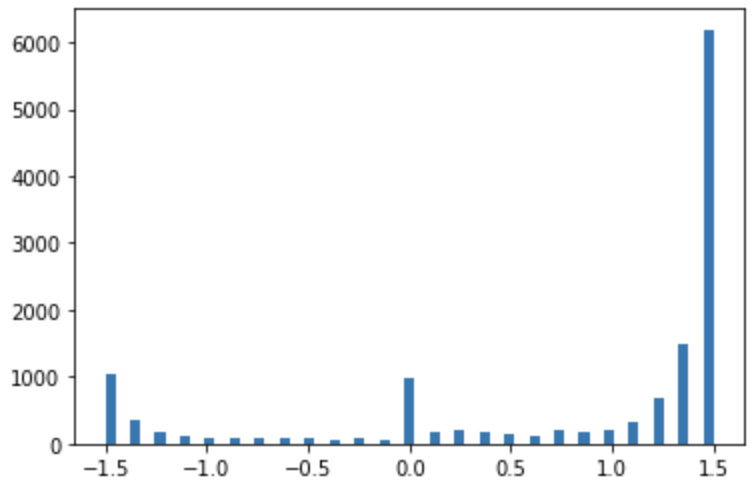
The histogram shows spikes at the min, max and 0 steering command values. This reflects the nature of the course which consists of straightaways and a few sharp turns. The positive values occur at a much higher frequency since the course was mostly right-hand turns.

We can normalize this distribution to have a more uniform distribution. This will ensure that the ML model is trained on a variety of inputs and doesn’t overfit to making just right-hand turns since that’s the majority of this dataset.

If the hist checkbox is selected, the dataset is pruned so that no more than a certain number of entries exist per bin. This value is set using the samples_per_bin variable and is default to 200.

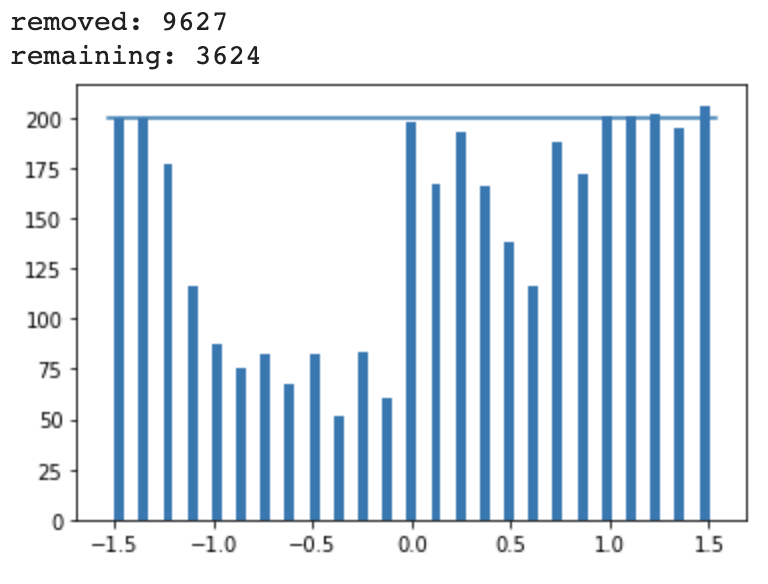
Over 9,000 samples were removed and around 3,600 entries remain. The histogram of the remaining entries is plotted, which looks much more uniform than the original histogram.

Image Preprocessing

Once the dataset is normalized, we can move on to evaluating the quality of the images by visualizing them. There are several steps we will take to process the images.

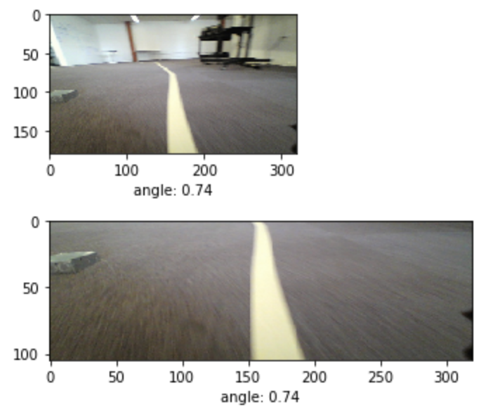
First, we will resize the images from their native 640×480 to 320×180. While this does reduce the resolution, the details that we will lose in the images aren’t valuable for this task. The smaller image significantly reduces the number of parameters in the model and makes the training process much faster.

We will also crop the image to remove regions of the image that aren’t relevant to the training task. This task is primarily concerned with the location of the track in the image. The portions of the image which don’t contain the floor and the track aren’t relevant and can be removed. This prevents the model from learning features that are unique to the environment.

The image below shows the original image, resized to 320×180, as well as the cropped version. The cropped image retains the floor and lane while removing the rest of the office environment.

We will incorporate these image processing functions into subsequent steps in the ML model definition and training process.

Define Training and Validation Datasets

Once the dataset is processed and reviewed, we need to split that data into a training set and a validation set. The training set is the data that is used to adjust the weights of the model during training. The validation set doesn’t impact the model weights but is used to verify that the model isn’t overfitting on the training data.

Image Augmentation

Before splitting the dataset, we will explore data augmentation. Since our dataset is relatively small, we can use data augmentation techniques to generate slightly modified versions of our dataset for training and vastly expand the dataset. This can make the final model more accurate and more robust to changes in the environment.

Keras provides the ImageDataGenerator class which has several built-in functions for manipulating images. This includes shifting the image vertically or horizontally, zooming in on the image, or adjusting the brightness. The post, “Exploring Image Data Augmentation with Keras and Tensorflow” provides a good overview of the options with examples of each. Some examples of augmentations of images from the dataset are shown below.

Data Generator Development

When working with large datasets, it’s helpful to use Keras data generators to handle loading the data. These are specifically helpful when manipulating datasets containing images. For this example, we will define our own basic data generator. In the future, we can use the Keras implementations such as the ImageDataGenerator class.

Our data generator will take in a dataset of sample data as well as the batch size hyperparameter value and a flag to determine if the data should be augmented.

def generator(samples, batch_size=32, aug=0)

The data generator begins by loading a specific set of data from the samples based on the batch size

batch_samples = samples[offset:offset + batch_size]

For each sample, it loads an image and resizes it.

center_image = cv2.imread(name)
center_image = cv2.resize( center_image, (320, 180))

It then loads the steering angle associated with that image.

angle = float(batch_sample[4])

If the aug flag is enabled, we perform basic image augmentation using our augmentation data generator.

it = datagen.flow(sample, batch_size=1)

We also potentially flip the image as well as the steering angle value.

flip_image = np.fliplr(center_image) 
flip_angle = -1 * angle

With or without augmentation, the image and the angle are then stored in unique arrays:

images.append(center_image) 
angles.append(angle)

Lastly, we shuffle and return the arrays.

yield sklearn.utils.shuffle(X_train, y_train)

Initialize the Training and Validation Datasets

Next, we use the train_test_split function from the sklearn library to split our dataset into training and validation samples.

train_samples, validation_samples = train_test_split(samples, test_size=0.2)

We use 80% of the data for training and 20% for validation. This ends up being around 2,900 training samples and 700 validation samples.

These are input into our dataset generator function resulting in a training data generator and a validation data generator.

train_generator = generator(train_samples, batch_size=batch_size_value, aug=1)
validation_generator = generator(validation_samples, batch_size=batch_size_value, aug=0)

Model Architecture and Training

For this application, we will use the model developed by Nvidia and described in their blog post, “End-to-End Deep Learning for Self-Driving Cars.” The model is defined in their paper, “End to End Learning for Self-Driving Cars.” They develop a convolutional neural network (CNN) to map raw pixels from a single front-facing camera directly to steering commands.

The network consists of 9 layers, including a normalization layer, 5 convolutional layers and 3 fully connected layers. A visualization of the model from the paper is shown below:

Compile the Model

This model is compiled using the following Keras functions. We trim the input image using the cropping values we discovered previously. We also ensure that the input image has a 180×320 resolution.

model.add(Cropping2D(cropping=((height_min,0), (width_min,0)), input_shape=(180,320,3)))

We also perform some basic preprocessing of the incoming data. We normalize the image values centered around zero with a small standard deviation.

model.add(Lambda(lambda x: (x / 255.0) - 0.5))

The remaining lines define the specific model layers.

Once the model is defined, we compile the model.

model.compile(loss='mse', optimizer=Adam(lr=0.001), metrics=['mse','mae','mape','cosine'])

We specify that we will use the Mean Squared Error for the loss function that we want to minimize during training. This metric is useful for regression tasks. We also specify that we want to use the Adam optimizer.

This results in a model with 15,004,791 trainable parameters.

Setup Callback Utilities

Callbacks are utility functions that are triggered and called during the model training process.

We first set up checkpoints. This is useful if you are doing long training sessions. It stores the model weights when the performance improves. If something happens during training, you can re-load the most successful model and re-start training. This is useful in the Colab environment because the instances can disconnect after a certain timeout period.

checkpoint = ModelCheckpoint(filepath, monitor='val_loss', verbose=1, save_best_only=True, mode='auto', period=1)

The weights will be stored in the model folder on the Colab instance.

Next, we use the EarlyStopping callback to end the training process if the model performance plateaus. This helps prevent overfitting.

early_stop = EarlyStopping(monitor='val_loss', patience=10)

The ReduceLROnPlateau function is similar. If the model performance stops improving, the learning rate of the Adam optimizer is automatically adjusted.

reduce_lr = ReduceLROnPlateau(monitor='val_loss', factor=0.2, patience=5, min_lr=0.001)

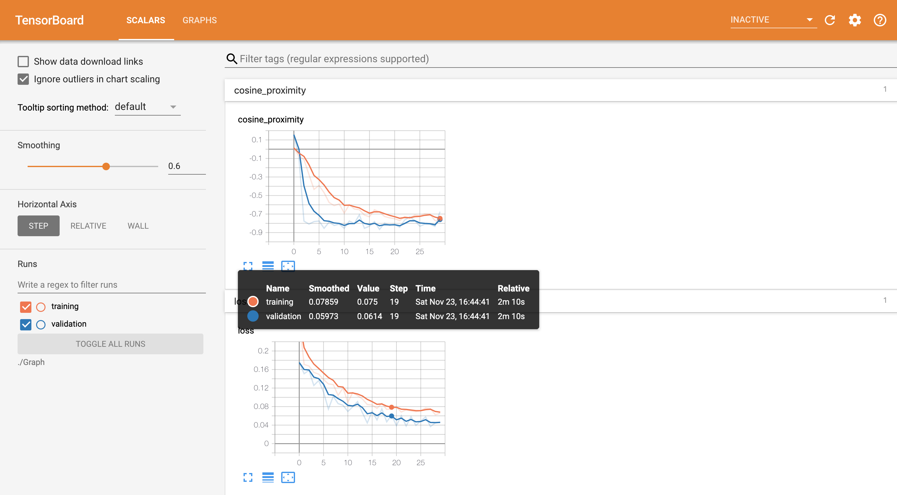
Lastly, we set up Tensorboard. TensorBoard is a visualization tool provided with TensorFlow. It enables tracking experiment metrics like loss and accuracy as well as visualizing the model graph. When executing the cell, a link is provided in the output to the Tensorboard instance. An example image of Tensorboard during the training process is shown below.

Train the Model

Once the model is compiled and the set of callbacks defined, we can start the training process. First, we set the hyperparameters.

We define the step sizes for the training and validation data.

steps_per_epoch=(len(train_samples) / batch_size_value)
validation_steps=(len(validation_samples) / batch_size_value)

This defines the total number of steps (batches of samples) to yield from the data generator before declaring one epoch finished and starting the next epoch.

Next, we set the number of epochs.

n_epoch = 50

Finally, we use the fit_generator function to start the model training process.

history_object = model.fit_generator(
generator=train_generator,
steps_per_epoch=STEP_SIZE_TRAIN,
validation_data=validation_generator,
validation_steps=STEP_SIZE_VALID,
callbacks=callbacks_list,
use_multiprocessing=True,
epochs=n_epoch)

Once training begins, the cell will output the metrics for each epoch. Once training is complete, the model can be saved to the Colab instance for download to a local workstation.

Model Evaluation

The model training process provides some insight into the model’s performance via the performance metrics that are output. However, to better understand how the model will perform, we can use the trained model to make predictions on some of our sample data and view the results.

Model Training Statistics

First, we can visualize the performance of the model by plotting the loss function for both the training and validation datasets during the training process.

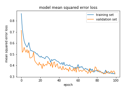
Here we can see the loss drops quickly in the beginning but the improvement slows as the training process continues. Both the training and validation plots are similar, indicating we are not overfitting on the data.

View Prediction Statistics

We can also load a subset of the dataset and predict steering values for each of the images in the subset of data. We can compare the predicted values to the known true values and visualize the error.

First, we bin the error between the predicted and true steering commands for each image and plot a histogram.

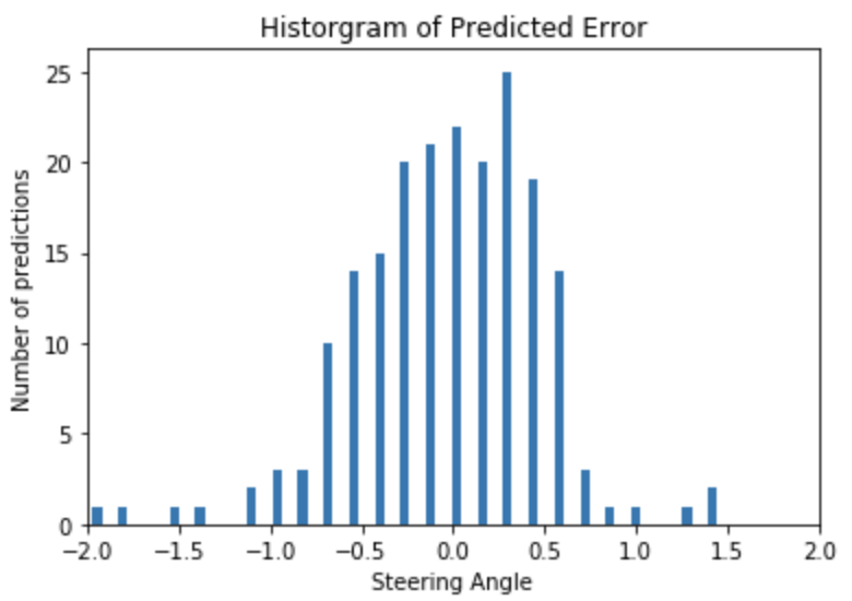
The error seems to be pretty evenly distributed with the majority of the errors near 0 which is good.

We can also visualize a scatter plot of the predicted values with the known values.

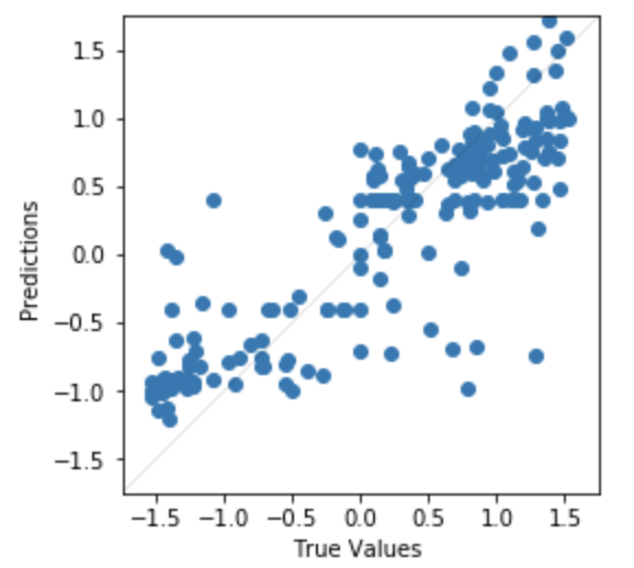
Here we can see the model performs better at the minimum and maximum steering angles than the middle.

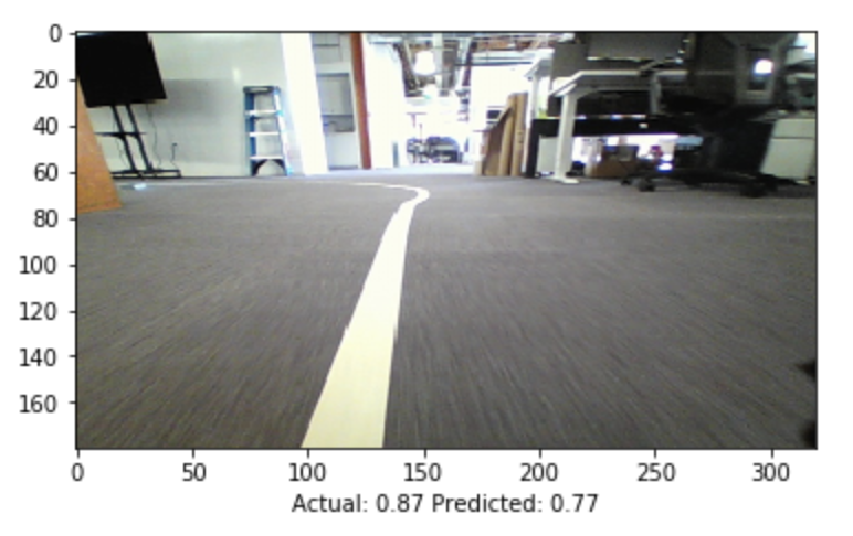
View Prediction Images

We can also look at individual images to get a sense of the model’s performance. The image below shows both the precited and true steering angle for a single image.

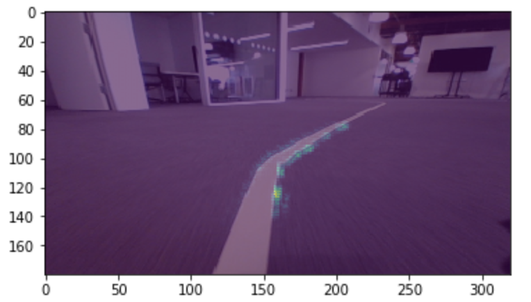
We can also use the visualize_saliency function to generate a heatmap indicating the regions of the image that most contribute towards the model output.

Saliency maps were introduced in the paper Deep Inside Convolutional Networks: Visualising Image Classification Models and Saliency Maps. They are based on gradients and they calculate the gradient of the output with respect to each pixel in the input image. This tells us how the output changes with respect to small changes in the input image pixels.

grads = visualize_saliency(model,
layer_idx,
filter_indices=None,
seed_input=sample_image_mod,
grad_modifier='absolute',
backprop_modifier='guided')

In the example image below, we see that the network is most sensitive to pixels near the lane marking.

Model Deployment

Once the model was trained, it was placed on the embedded device and integrated into the RC car control system. The model predicted steering commands in real-time based on input images from the webcam.

The video below depicts a completely autonomous lap using the model defined in this process. The image recorded by the webcam can be seen as well as an overlay of the saliency image depicting the areas in the image that most contribute towards the steering command output.